week5
Links
Code
- lsys1.tar.gz -- the first L-system
code, interprets a simple L-system as frequency vs. time
- lsys2.tar.gz -- L-systems with
very short time-scales; individual sound events
- lsys3.tar.gz -- L-systems interpreted
by unfolding an array of pitches, moving rectangle determines
the notes in the chord
- lsys4.tar.gz -- L-systems interpreted
as they are drawn
Before we got into Lindenmayer Systems (L-systems), we finished
a bit of business from last week's room and space simulation
lecture. Francisco showed off some snazzy impulse-respsonse
convolution examples, using
soundhack and several
downloaded impulse response files from the web (see
last week
for links to a few sites). Convolution is a really powerful tool
for recreating the sound of a particular space.
Next Brad described a newer approach using a technique called finite element
simulation, where sound is communicated through a virtual
grid of interconnected objects -- each one might represent a "packet"
of air (or individual air molecules themselves if the finite elements
in the grid were thought to be small enough). Each element has a small
delay line associated with it, possibly also with a gentle filter, that
represents what happens to a propogating sound waveform as it traverses
the "packet" of air for the element.
 This technique allows for a wide range of simulated space topologies as
well as the potential for placing various reflective or absorptive objects
within it. It is extremely computationally expensive, however, and
the shape of the grid does have a strong effect on the resulting sound.
It's interesting to consider, though.
This technique allows for a wide range of simulated space topologies as
well as the potential for placing various reflective or absorptive objects
within it. It is extremely computationally expensive, however, and
the shape of the grid does have a strong effect on the resulting sound.
It's interesting to consider, though.
We do have a physical model instrument that implements a very small
finite element simulation (called a "mesh" in this case) -- the
MMESH2D
instrument based on work by Smith and Van Duyne (from Perry Cook's
STK code). The instrument is excited by an impulse at one of the nodal
points in the mesh, creating a wide variety of 'struck metal' kinds of
sounds. It shouldn't be too hard to modify for audio input.
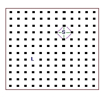
And Then the L-systems
Lindenmayer Systems (L-systems), developed by Aristid
Lindenmayer to model biological growth processes, produce output
that is quite musically suggestive. Unfortunately there is a tendency
to look at the produced graphs of an L-system and imagine a fairly
straightfoward translation onto particular musical parameters, which
may or may not produce snazzy music.
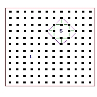
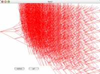
L-system1
In our first little experiment, we did the obvious -- designed a simple
L-system and interpreted it as frequency (the height of the graphic) vs. time.
Each little time-slice through the graph was about 0.1 seconds, so the sound
evolved over 20-30 seconds.
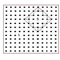
L-system2
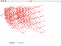
Next we decided to have some fun with the time-scale. Imagining the L-system
graph more as an FFT of a single sonic event, we moved the interpretation
of the x-axis from 0.1 seconds/pixel to 0.01 or even 0.001 seconds/pixel.
This resulted in much shorter duration sounds:
- lsys2a.mp3 -- 3.5 second realization,
5 levels of recursion
- lsys2b.mp3 -- 7.1 second realization,
9 levels of recursion (very dense!)
- lsys2c.mp3 -- 0.65 second realization,
5 levels of recursion
- lsys2d.mp3 -- 0.4 second realization,
5 levels of recursion
The last two have a rather pronounced high-frequency component that does not
arise from the L-systems we generated. Instead, it is an artifact of the
very small 'window' size we used to generate the sound. Still kind of
fun to hear.
Just for the heck of it, we then went back 'the other way' with our last
L-system and generated long realizations. For the longest, we replaced
the sine wave we were using for each pixel/frequency value with
a square wave. Oh it was a thrill!
- lsys2e.mp3 -- 6 second realization,
5 levels of recursion
- lsys2f.mp3 -- 60 second realization,
5 levels of recursion
- lsys2g.mp3 -- 60 second realization,
5 levels of recursion, square waves
All three of the aboce sounds come from the same L-system, and in fact
it is the same that we used to generate the lsys2d.mp3 file.
The square wave version has some nifty foldover happening.
L-system3
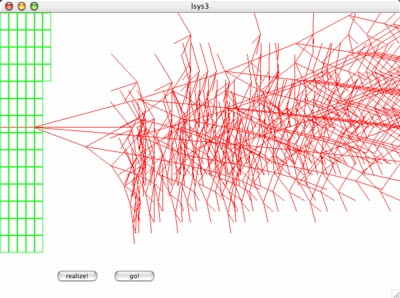
For our next L-system interpretation, we moved away from an obvious
frequency vs. time graph to a system that unfolded an array of pitches,
forming chrords depending on how many graph-system lines were in a moving
rectangle. The real fun came when we used the
MMODALBAR
physical model instrument as our sonic generator.
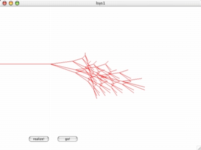
L-system4
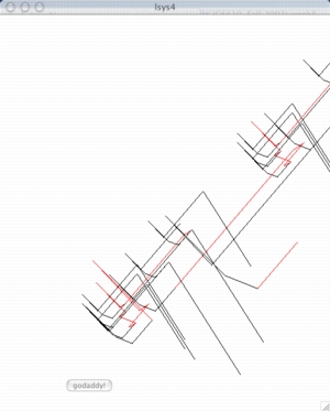
Finally, we designed a simple model that unfolded and interpreted an L-system
simultaneously, capturing the trajectory of the graph as a music generating
algorithm (this is similar to the way we interpreted the
Lorenz attractor
in a previous class. The code contains several variations on this,
interpreting the x and y axes as frequency, amplitude, timber, etc.
We also used a number of different instruments for the data interpretation,
showing that any combination of parameters can be mapped from an L-system
onto a sound-producing algorthim. Use your imagination!
One caveat -- the "L-systems" we coded into our little demos are very
simplistic, and they only follow the "bare bones" of how contemporary
researchers think of L-systems. We don't use the flexible
recursive grammar for specifying and controlling
an L-system; instead we imbedded an L-system recursion in a simple
function call or two.
Next week Luke Dubois will show his L-system work. Luke does draw
heavily upon the use of a recursive grammar. It's a very powerful
technique. See the links at the top of the page for a better view
of current L-systems research.