|
| <-- Back to Previous Page | TOC | Next Section --> |
Chapter 2: The Digital Representation of Sound,
|
||
|
The distinction between analog and digital information is not an easy one to understand, but it’s fundamental to the realm of computer music (and in fact computer anything!). In this section, we’ll offer some analogies, explanations, and other ways to understand the difference more intuitively. Imagine watching someone walking along, bouncing a ball. Now imagine that the ball leaves a trail of smoke in its path. What does the trail look like? Probably some sort of continuous zigzag pattern, right?
Figure 2.4 The path of a bouncing ball. OK, keep watching, but now blink repeatedly. What does the trail look like now? Because we are blinking our eyes, we’re only able to see the ball at discrete moments in time. It’s on the way up, we blink, now it’s moved up a bit more, we blink again, now it may be on the way down, and so on. We’ll call these snapshots samples because we’ve been taking visual samples of the complete trajectory that the ball is following. The rate at which we obtain these samples (blink our eyes) is called the sampling rate. It’s pretty clear, though, that the faster we sample, the better chance we have of getting an accurate picture of the entire continuous path along which the ball has been traveling.
Figure 2.5 The same path, but sampled by blinking. What’s the difference between the two views of the bouncing ball: the blinking and the nonblinking? Each view pretty much gives the same picture of the ball’s path. We can tell how fast the ball is moving and how high it’s bouncing. The only real difference seems to be that in the first case the trail is continuous, and in the second it is broken, or discrete. That’s the main distinction between analog and digital representations of information: analog information is continuous, while digital information is not. |
||
|
|
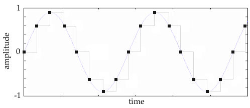
Analog and Digital Waveform RepresentationsNow let’s take a look at two time domain representations of a sound wave, one analog and one digital, in Figure 2.6.
Figure 2.6 An analog waveform and its digital cousin: the analog waveform has smooth and continuous changes, and the digital version of the same waveform has a stairstep look. The black squares are the actual samples taken by the computer. The grey lines suggest the "staircasing" that is an inevitable result of converting an analog signal to digital form. Note that the grey lines are only for show—all that the computer knows about are the discrete points marked by the black squares. There is nothing in between those points. The analog waveform is nice and smooth, while the digital version is kind of chunky. This "chunkiness" is called quantization or staircasing—for obvious reasons! Where do the "stairsteps" come from? Go back and look at the digital bouncing ball figure again, and see what would happen if you connected each of the samples with two lines at a right angle. Voila, a staircase! Staircasing is an artifact of the digital recording process, and it illustrates how digitally recorded waveforms are only approximations of analog sources. They will always be approximations, in some sense, since it is theoretically impossible to store truly continuous data digitally. However, by increasing the number of samples taken each second (the sample rate), as well as increasing the accuracy of those samples (the resolution), an extremely accurate recording can be made. In fact, we can prove mathematically that we can get so accurate that, theoretically, there is no difference between the analog waveform and its digital representation, at least to our ears. |
| <-- Back to Previous Page | Next Section --> |
©Burk/Polansky/Repetto/Roberts/Rockmore. All rights reserved.