|
| <-- Back to Previous Page | TOC | Next Section --> |
Chapter 2: The Digital Representation of Sound,
|
||
|
The world is continuous. Time marches on and on, and there are plenty of things that we can measure at any instant. For example, weather forecasters might keep an ongoing record of the temperature or barometric pressure. If you are in the hospital, the nurses might be keeping a record of your temperature, your heart rate, or your brain waves. Any of these records gives you a function f(t) where, at a given time t, f(t) is the value of the particular statistic that interests you. These sorts of functions are called time series.
Figure 2.1 Genetic algorithms (GA) are evolutionary computing systems, which have been applied to things like optimization and machine learning. These are examples of continuous functions. What we mean by "continuous" is that at any instant of time the functions take on a well-defined value, so that they make squiggly line graphs that could be traced without the pencil ever leaving the paper. This might also be called an analog function. Of course, the time series that interest us are those that represent sound. In particular, we want to take these time series, stick them on the computer, and play with them! Now, if you’ve been paying attention, you may realize that at this moment we’re in a bit of a bind: the type of time series that we’ve been describing is a continuous function. That is, at every instant in time, we could write down a number that is the value of the function at that instant—whether it be how much your eardrum has been displaced, what your temperature is, what your heart rate is, and so on. But such a continuous function would provide an infinite list of numbers (any one of which may have an infinite expansion, like So how do we do it? How can we represent sound as a finite collection of numbers that can be stored efficiently, in a finite amount of space, on a computer, and played back and manipulated at will? In short, how do we represent sound digitally? That’s the problem that we’ll start to investigate in this chapter. Somehow we have to come up with a finite list of numbers that does a good job of representing our continuous function. We do it by sampling the original function, at every few instants (at some predetermined rate, called the sampling rate), recording the value of the function at that moment. For example, maybe we only record the temperature every 5 minutes. For sound we need to go a lot faster, and we often use a special device that grabs instantaneous amplitudes at rapid, audio rates (called an analog to digital converter, or ADC). A continuous function is also called an analog function, and, to restate the problem, we have to convert analog functions to lists of samples, or digital functions, which is the fundamental way that computers store information. In computers, think of a digital function as a function of location in computer memory. That is, these functions are stored as lists of numbers, and as we read through them we are basically creating a discrete function of time of individual amplitude values.
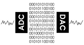
Figure 2.2 A pictorial description of the recording and playback of sounds through an ADC/DAC. In analog to digital conversions, continuous functions (for example, air pressures, sound waves, or voltages) are sampled and stored as numerical values. In digital to analog conversions, numerical values are interpolated by the converter to force some continuous system (such as amplifiers, speakers, and subsequently the air and our ears) into a continuous vibration. Interpolation just means smoothly transitioning across the discrete numerical values. When we digitally record a sound, an image, or even a temperature reading, we numerically represent that phenomenon. To convert sounds between our analog world and the digital world of the computer, we use a device called an analog to digital converter (ADC). A digital to analog converter (DAC) is used to convert these numbers back to sound (or to make the numbers usable by an analog device, like a loudspeaker). An ADC takes smooth functions (of the kind found in the physical world) and returns a list of discrete values. A DAC takes a list of discrete values (like the kind found in the computer world) and returns a smooth, continuous function, or more accurately the ability to create such a function from the computer memory or storage medium.
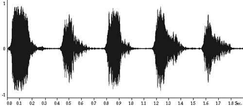
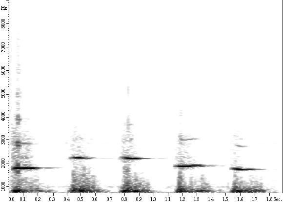
Figure 2.3 Two graphical representations of sound. The top is our usual time domain graph, or audiogram, of the waveform created by a five-note whistled melody. Time is on the x-axis, and amplitude is on the y-axis. We’ll be giving a much more precise description of the frequency domain in Chapter 3, but for now we can simply think of sounds as combinations of more basic sounds that are distinguished according to their "brightness." We then assign numbers to these basic sounds according to their brightness. The brighter a sound, the higher the number. As we learned in Chapter 1, this number is called the frequency, and the basic sound is called a sinusoid, the general term for sinelike waveforms. So, high frequency means high brightness, and low frequency means low brightness (like a deep bass rumble), and in between is, well, simply in between. All sound is a combination of these sinusoids, of varying amplitudes. It’s sort of like making soup and putting in a bunch of basic spices: the flavor will depend on how much of each spice you include, and you can change things dramatically when you alter the proportions. The sinusoids are our basic sound spices! The complete description of how much of each of the frequencies is used is called the spectrum of the sound. Since sounds change over time, the proportions of each of the sinusoids changes too. Just like when you spice up that soup, as you let it boil the spice proportion may be changing as things evaporate. |
| <-- Back to Previous Page | Next Section --> |
©Burk/Polansky/Repetto/Roberts/Rockmore. All rights reserved.