One of the first steps toward high-level analysis of audio recordings is decomposing the signal into a representation that can be easily digested by a computer. A more or less standard approach is to carve up the signal into a sequence of small frames (say, 50ms long), and then extracting some features from each frame, such as chroma/pitch distributions, or timbre/Mel-frequency cepstral coefficients.
One of the things that I’ve been working on is learning audio features which are informed by commonly used instrumentation in jazz recordings. The idea here is that if we can decompose a song into its constituent instruments — even approximately — it may be easier to detect high-level patterns, such as repetitions, instrument solos, etc. Lofty goals, indeed!
As a first step in this direction, I gathered the RWC Instrument Database, and extracted recordings of all the instruments we’re likely to encounter in any given jazz recording. These instrument recordings are extremely clean: one note at a time, in a controlled environment with almost no ambient noise. So it’s not exactly representative of what you’d find in the wild, but it’s a good starting point under nearly ideal conditions.
Each recording was chopped up into short frames (~46ms), and each frame was converted into a log-amplitude Mel spectrogram in  .
.
Given this collection of instrument-labeled audio frames, my general strategy will be to learn a latent factorization of the feature space so that each frame can be explained by relatively few factors.
If we assume that the factors (the codebook)  are already known, then an audio frame
  can be encoded via non-negative sparse coding:
![\[ f(x_t \given D, \lambda) := \argmin_{\alpha\in\R_+^{k}} \frac{1}{2}\|x_t - D\alpha\|^2 + \lambda \|\alpha\|_1, \]](wp-content/ql-cache/quicklatex.com-30fee851b748fd5dfd32aa5aad4b1e20_l3.png "Rendered by QuickLaTeX.com")
where  is a parameter to control the amount of desired sparsity in the encoding
  .
.
Of course, we don’t know  yet, so we’ll have to learn it. We can do this on a per-instrument level by grouping all the
  audio frames
  associated with the
  th instrument, and alternately solving the following problem for both
  and
and  :
:
![\[ \min_{D^I, \alpha_{1,2,\dots,n}^I} \sum_{t=1}^n \|x_t^I - D^I \alpha_t^I\|^2 + \lambda\|\alpha_t^I\|_1. \]](wp-content/ql-cache/quicklatex.com-3a5ffa2ad8ce8723caa68382b0f97085_l3.png "Rendered by QuickLaTeX.com")
After doing this independently for each instrument, we can collect each of the codebooks into one giant codebook . In my experiments, I’ve been allowing 64 basis elements for most instruments, and 128 for those with high octave range (piano, vibraphone, etc). The resulting has around 2400 elements.
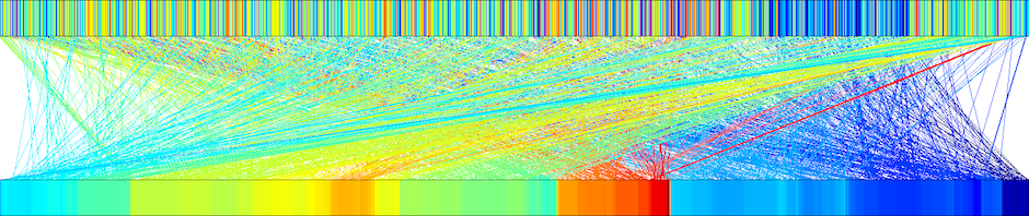
It can be difficult to discern much from visual inspection of thousands of codebook elements, but some interesting things happen if we plot the correlation between the learned features across instruments:

Not quite surprisingly, there’s a large amount of block structure in this figure. Let’s zoom in on few interesting regions. First up, the upper-left block:

From this, we can see that piano, electric piano, vibraphone, and flute might be difficult to tease apart, but both acoustic and electric guitar separate nicely. Note that the input features here have no notion of dynamics, such as attack and sustain, which may help explain the collision of flute with piano and vibes. [Future work!]
The picture is much clearer in the middle block, where instruments seem to separate out by their range and harmonics. Note that violin still collides with piano and vibes (not pictured).

Finally, the lower-right block includes a variety of instruments, percussion, and human voice. With the exception of kick/toms, it’s largely an undifferentiated mess:

It seems a bit curious that cymbals show such strong correlations with almost all other instruments. One possible explanation is that most instrument codebooks will need to include at least one component that models broad-band noise; but cymbals are almost entirely broad-band noise. So, although the basis elements themselves appear ambiguous, it may be that the encodings derived from them are still interpretable: at least, interpretable by a clever learning algorithm. More on this as it develops…