Again, look at last week and the previous week to see what has led up to this point in the class.
But first, Luke showed off the new Curtis Roads book
Microsound, filled with loads of informative information
informing us about informated sound-creation. Go
to
barnesandnoble.com to order it,
or you can also visit
the
emf book page if you want to help support the good folks at
The Electronic Music Foundation.
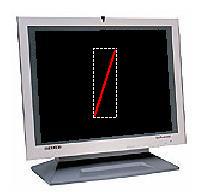
We wanted to find a way to control the 'scrolling' through the FFT using some kind of external interface, i.e. not a mouse or graphics tablet or other such technology. In a veritable stroke of genius, Luke hit upon the idea of using a laser pointer against a black background to determine the FFT frame value for resynthesis. The amazingly appropriate aspect is that the only handy black-background surface we could find was the shell of an old NeXT "pizza-box" computer. Hi! This is Steve Jobs! The red against the black was good because it provided an excellent color contrast for the camera-tracking software.
Looking for color is a relatively easy was to track "external" stuff, although you have to be careful because the color can shift depending on lighting conditions. The more contrast between your background and foreground (tracked) colors, the better. Also, we will be looking for a range of color in our tracker, because this will allow for a bit of lighting 'fuzziness'. If you do design an application for real-world use that relies upon color tracking, be sure not to hard-code the color into the app. Leave it able to be recalibrated in the context(s) where you will be using it.
Using our digital cameras (room 313 has a nice setup for this kind of work), we connect the "DV" output through the firewire port and use
With image date streaming in through the jit.qt.grab object, we can use the
The handy MSP "vexpr" object works like "expr" only can operate on arrays:
However, the best approach would be for us not to define in advance the color we want to track, but to grab it from the incoming camera signal -- that way we will know how the color appears in the place where we use the application. The little "syringe" object on the Max/MSP/jitter palette does this. We can use it to grab a color from the incoming signal as displayed on the screen, and by connecting it's output to the "vexpr" object we can convert from the 0-255 values to the 0.0-1.0 values for the colors. We can also use "vexpr" to through in a range-calculation, so that we don't get too narrowly focused on one color value. The class patch shows this.
jit.findbounds puts out lists of maximum and minimum boundary values for the bounding box. The ever-useful "unpack" object will convert these to x & y coordinate values. Just for fun, Luke hooked them directly to the "qtmusic" object playing that vibrant QuickTime piano sound -- the coordinate values were mapped onto MIDI amplitude and note-number values. It was more fun than a barrel of monkeys.
With a little more math, we also connected the output of this little system directly to an oscillator to see how much latency was in the patch -- how closely did it track the movement of the laser pointer? All agreed it was quite good. Yes, quite good. It felt good. Good.
Because we are tracking a red line against a black background, we modified out original use of jit.findbounds to just look at the red component. This is for efficiency (we don't need to track the G and B color components). jit.unpack did the trick again.
Then we used the jit.lcd object to combine our bounding-box tracking with the incoming video signal, to create a BigEye kind of system, but one we can use easily within Max/MSP/jitter. We had some minor difficulties to resolve concerning the synchronization of the lcd drawing, the frame rate of incoming frames, and the clearing of the lcd to update the image. Using the "trigger" ("t") Max object allowed us to sync all our bangs... god, this language...
In general, if you are using several "metro" objects to repeatedly trigger events (especially with a tight timing), it is good to try to combine them into a single master "metro" clock -- efficiency is better + your events will be syncronized.
After putting all this stuff together, it worked! One thing we will
have to keep in mind is that the bounding box coordinates may or may
not map onto the number of FFT data frames we have. Scaling, scaling,
over the bounding main... (ha ha! I just made that up!).
We will probably be revisiting OpenGL later in the class. In the meantime, here are a few links to some good OpenGL sites:
Anyhow, the
Aside: just FYI, the jit.gl.* objects actually use jitter matrices to communicate with each other. I doubt you will ever have to access this data, but it does show the flexibility of the jitter matrix setup for doing arbitrary data massaging. In fact, one of the potentially cute uses of jit.findbounds is to operate on non-graphic data. Think about it...
As with the jit.qt.movie or jit.qt.grab objects. the jit.gl.render object works by getting banged. It renders a new scene everytime it gets a Max bang. Generally you will want to erase the previous scene before new rendering, but you can get some cool overlay effects by not doing this.
There's a lot of GL material imbedded in jitter; certainly more than we can cover here. The best way to learn this is to hit the tutorials, plus scope the web sites above, etc. It is a very powerful standard.
What we plan to do is fairly simple, though. But even something as simple as our use shows the power of OpenGL -- you get a lot of really fancy-looking stuff for very little effort. We plan to use a "texture", and we will modify the "texture" in one dimension to reflect the peaks in the FFT data.
What does this mean? Well, a "texture" is basically a flat set of 2-D graphics data (our sonogram!) that you can put on an OpenGL object. In our case, we plan to put the sonogram "texture" onto a flat plane, BUT we plan to warp the plane (using an OpenGL technique called an 'extrusion map') along one axis to show the amplitude peaks in the FFT spectrum.
Here's a quick outline of what we do:
Check out the class patches for the finished version.