|
| <-- Back to Previous Page | TOC | Next Section --> |
Chapter 5: The Transformation of Sound by ComputerSection 5.6: Morphing
|
||
In recent years the idea of morphing, or turning one sound (or image) into another, has become quite popular. What is especially interesting, besides the idea of having a lion roar change gradually and imperceptibly into a meow, is the broader idea that there are sounds "in between" other sounds.
Figure 5.15 Image morphing: several stages of a morph. What does it mean to change one sound into another? Well, how would you
graphically change a picture into another? Would you replace, over time,
little bits of one picture with those of another? Would you gradually
change the most important shapes of one into those of the other? Would
you look for important features (background, foreground, color, brightness,
saturation, etc.), isolate them, and cross-fade them independently? You
can see that there are lots of ways to morph a picture, and each way produces
a different set of effects. The same is true for sound. |
||
|
|
||
|
|
Larry Polansky's "51 Melodies" is a terrific example of a computer-assisted composition that uses morphing to generate novel (and kind of insane!) melodies. Polansky specified the source and target melodies, and then wrote a computer program to generate the melodies in between. From the liner notes to the CD "Change": "51 Melodies is based on two melodies, a source and a target, and is in three sections. The piece begins with the source, a kind of pseudo-anonymous rock lick. The target melody, an octave higher and more chromatic, appears at the beginning of the third section, played in unison by the guitars and bass. The piece ends with the source. In between, the two guitars morph, in a variety of different, independent ways, from the source to the target (over the course of Sections 1 and 2) and back again (Section 3). A number of different morphing functions, both durational and melodic, are used to distinguish the three sections." (The Soundfile 5.22 is an three minute edited version of the complete 12 minute piece, composed of one minute sections from the beginning, middle, and end of the recording.) |
|
|
|
||
Simple MorphingThe simplest sonic morph is essentially an amplitude cross-fade. Clearly, this doesn’t do much (you could do it on a little audio mixer). |
||
|
|
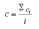
Figure 5.16 An amplitude cross-fade of a number of different data points. What would constitute a more interesting morph, even limiting us to the time domain? How about this: let’s take a sound and gradually replace little bits of it with another sound. If we overlap the segments that we’re "replacing," we will avoid horrible clicks that will result from samples jumping drastically at the points of insertion. Interpolation and Replacement MorphingThe two ways of morphing described above might be called replacement and interpolation morphing, respectively. In a replacement morph, intact values are gradually substituted from one sound into another. In an interpolation morph, we compare the values between two sounds and select values somewhere between them for the new sound. In the former, we are morphing completely some part of the time; in the latter, we are morphing somewhat all of the time. In general, we can specify a degree of morphing, by convention called Ω, that tells how far one sound is from the other. A general formula for (linear) interpolation is: I = A + (Ω*(B – A)) In this equation, A is the starting value, B is the ending value, and Ω is the interpolation index, or "how far" you want to go. Thus, when Ω = 0, I = A; when Ω = 1, I = B, and when Ω = 0.5, I = the average of A and B. This equation is a complicated way of saying: take some sound (SourceSound) and add to it some percentage of the difference between it and another sound (TargetSound – SourceSound), to get the new sound. Sonic morphing can be more interesting in the frequency domain, in the creation of sounds whose spectral content is some kind of hybrid of two other sounds. (Convolution, by the way, could be thought of as a kind of morph!) An interesting approach to morphing is to take some feature of a sound and morph that feature onto another sound, trying to leave everything else the same. This is called feature morphing. Theoretically, one could take any mathematical or statistical feature of the sound, even perceptually meaningless ones—like the standard deviation of every 13th bin—and come up with a simple way to morph that feature. This can produce interesting effects. But most researchers have concentrated their efforts on features, or some organized representation of the data, that are perceptually, cognitively, or even musically salient, such as attack time, brightness, roughness, harmonicity, and so on, finding that feature morphing is most effective on such perceptually meaningful features. Feature Morphing Example: Morphing the CentroidMusic cognition researchers and computer musicians commonly use a measure of sounds called the spectral centroid. The spectral centroid is a measure of the "brightness" of a sound, and it turns out to be extremely important in the way we compare different sounds. If two sounds have a radically different centroid, they are generally perceived to be timbrally distant (sometimes this is called a spectral metric). Basically, the centroid can be considered the average frequency component (taking into consideration the amplitude of all the frequency components). The formula for the spectral centroid of one FFT frame of a sound is:
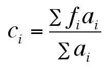
Ci is the centroid for one spectral frame, and i is the number of frames for the sound. A spectral frame is some number of samples that is equal to the size of the FFT. The (individual) centroid of a spectral frame is defined as the average frequency weighted by amplitudes, divided by the sum of the amplitudes, as follows:
We add up all the frequencies multiplied by their amplitudes (the numerator) and add up all the amplitudes (the denominator), and then divide. The "strongest" frequency wins! In other words, it’s the average frequency weighted by amplitude: where the frequency concentration of a sound is. |
|
|
|
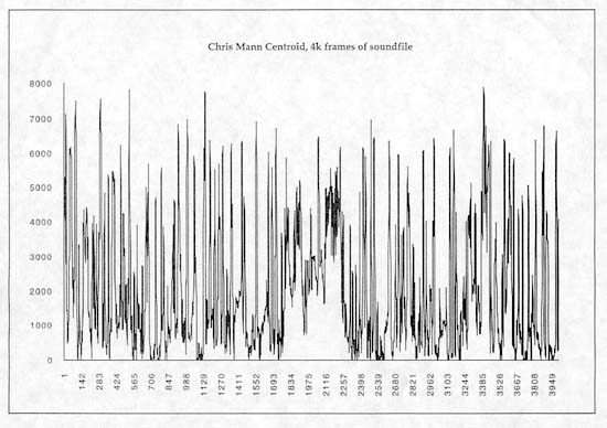
Figure 5.17 The centroid curve
of a sound over time. Note that centroids tend to be suprisingly high
and never the "fundamental" (unless our sound is a pure sine
wave). One of these curves is of a violin tone; the other is of a rapidly
changing voice (Australian sound poet Chris Mann). The soundfile for Chris
Mann is included as well. Now let’s take things one step further, and try to morph the centroid of one sound onto that of another. Our goal is to take the time-variant centroid from one sound and graft that onto a second sound, preserving as much of the second sound’s amplitude/spectra relationship as possible. In other words, we’re trying to morph one feature while leaving others constant. To do this, we can think of the centroid in an unusual way: as the frequency that divides the total sound file energy into two parts (above and below). That’s what an average is. For some time-variant centroid (ci) extracted from one sound and some total amplitude from another (ampsum), we simply "plop" the new centroid onto the sound and scale the amplitude of the frequency bins above and below the new centroid frequency to (0.5 * ampsum). This will produce a sort of "brightness morph." Notice that on either side of the centroid in the new sound, the spectral amplitude relationships remain the same. We’ve just forced a new centroid. |
|
| <-- Back to Previous Page | Next Section --> |
©Burk/Polansky/Repetto/Roberts/Rockmore. All rights reserved.