Chapter 4: The Synthesis of Sound by Computer

Section 4.9: Physical Modeling

We’ve already covered a bit of material on physical modeling without even telling you—the ideas behind formant synthesis are directly derived from our knowledge of the physical construction and behavior of certain instruments. Like all of the synthesis methods we’ve covered, physical modeling is not one specific technique, but rather a variety of related techniques. Behind them all, however, is the basic idea that by understanding how sound/vibration/air/string behaves in some physical system (like an instrument), we can model that system in a computer and thus synthetically generate realistic sounds.

Karplus-Strong Algorithm

Let’s take a look at a really simple but very effective physical model of a plucked string, called the Karplus-Strong algorithm (so named for its principal inventors, Kevin Karplus and Alex Strong). One of the first musically useful physical models (dating from the early 1980s), the Karplus-Strong algorithm has proven quite effective at generating a variety of plucked-string sounds (acoustic and electric guitars, banjos, and kotos) and even drumlike timbres.

Applet 4.13
Karplus-Strong plucked string algorithm

Fun with the Karplus-Strong plucked string algorithm.

Here’s a simplified view of what happens when we pluck a string: at first the string is highly energized and it vibrates like mad, creating a fairly complex (meaning rich in harmonics) sound wave whose fundamental frequency is determined by the mass and tension of the string. Gradually, thanks to friction between the air and the string, the string’s energy is depleted and the wave becomes less complex, resulting in a "purer" tone with fewer harmonics. After some amount of time all of the energy from the pluck is gone, and the string stops vibrating.

If you have access to a stringed instrument, particularly one with some very low notes, give one of the strings a good pluck and see if you can see and hear what’s happening per the description above.

How a Computer Models a Plucked String with the Karplus-Strong Algorithm

Now that we have a physical idea of what’s happening in a plucked string, how can we model it with a computer? The Karplus-Strong algorithm does it like this: first we start with a buffer full of random values—noise. (A buffer is just some computer memory (RAM) where we can store a bunch of numbers.) The numbers in this buffer represent the initial energy that is transferred to the string by the pluck. The Karplus-Strong algorithm looks like this:

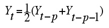
To generate a waveform, we start reading through the buffer and using the values in it as sample values. If we were to just keep reading through the buffer over and over again, what we’d get would be a complex, pitched waveform. It would be complex because we started out with noise, but pitched because we would be repeating the same set of random numbers. (Remember that any time we repeat a set of values, we end up with a pitched (periodic) sound. The pitch we get is directly related to the size of the buffer (the number of numbers it contains) we’re using, since each time through the buffer represents one complete cycle (or period) of the signal.)

Now here’s the trick to the Karplus-Strong algorithm: each time we read a value from the buffer, we average it with the last value we read. It is this averaged value that we use as our output sample. We then take that averaged sample and feed it back into the buffer. That way, over time, the buffer gets more and more averaged (this is a simple filter, like the averaging filter described in Section 3.1). Let’s look at the effect of these two actions separately.

Averaging and Feedback

First, what happens when we average two values? Averaging acts as a low-pass filter on the signal. Because we’re averaging the signal, the signal changes less with each sample, and by limiting how quickly it can change we’re limiting the number of high frequencies it can contain (since high frequencies have a high rate of change). So, averaging a signal effectively gets rid of high frequencies, which according to our string description we need to do—once the string is plucked, it should start losing harmonics over time.

The "over time" part is where feeding the averaged samples back into the buffer comes in. If we were to just keep averaging the values from the buffer but never actually changing them (that is, sticking the average back into the buffer), then we would still be stuck with a static waveform. We would keep averaging the same set of random numbers, so we would keep getting the same results.

Instead, each time we generate a new sample, we stick it back into the buffer. That way our waveform evolves as we move through it. The effect of this low-pass filtering accumulates over time, so that as the string "rings," more and more of the high frequencies are filtered out of it. The filtered waveform is then fed back into the buffer, where it is filtered again the next time through, and so on. After enough times through the process, the signal has been averaged so many times that it reaches equilibrium—the waveform is a flat line the string has died out.

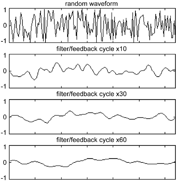
Figure 4.22  Applying the Karplus-Strong algorithm to a random waveform. After 60 passes through the filter/feedback cycle, all that’s left of the wild random noise is a gently curving wave.

The result is much like what we described in a plucked string: an initially complex, periodic waveform that gradually becomes less complex over time and ultimately fades away.

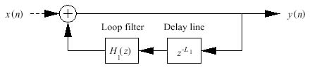
Figure 4.23  Schematic view of a computer software implementation of the basic Karplus-Strong algorithm.

For each note, the switch is flipped and the computer memory buffer is filled with random values (noise). To generate a sample, values are read from the buffer and averaged. The newly calculated sample is both sent to the output stream and fed back into the buffer. When the end of the buffer is reached, we simply wrap around and continue reading at the beginning. This sort of setup is often called a circular buffer. After many iterations of this process, the buffer’s contents will have been transformed from noise into a simple waveform.

If you think of the random noise as a lot of energy and the averaging of the buffer as a way of lessening that energy, this digital explanation is not all that dissimilar from what happens in the real, physical case.

Thanks to Matti Karjalainen for this graphic.

Physical models generally offer clear, "real world" controls that can be used to play an instrument in different ways, and the Karplus-Strong algorithm is no exception: we can relate the buffer size to pitch, the initial random numbers in the buffer to the energy given to the string by plucking it, and the low-pass buffer feedback technique to the effect of air friction on the vibrating string.

Soundfile 4.30
Super guitar

Many researchers and composers have worked on the plucked string sound as a kind of basic mode of physical modeling.

One researcher, engineer Charlie Sullivan (who we're proud to say is one of our Dartmouth colleagues!) built a "super" guitar in software. Here’s the heavy metal version of "The Star Spangled Banner."

Understand the Building Blocks of Sound

Physical modeling has become one of the most powerful and important current techniques in computer music sound synthesis. One of its most attractive features is that it uses a very small number of easy-to-understand building blocks—delays, filters, feedback loops, and commonsense notions of how instruments work—to model sounds. By offering the user just a few intuitive knobs (with names like "brightness," "breathiness," "pick hardness," and so on), we can use existing sound-producing mechanisms to create new, often fantastic, virtual instruments.

Soundfile 4.31
An example of
Perry Cook’s SPASM

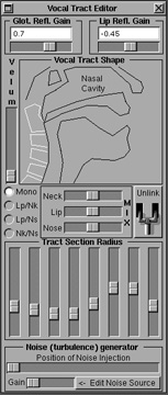
Figure 4.24  Part of the interface from Perry R. Cook’s SPASM singing voice software. Users of SPASM can make Sheila, a computerized singer, sing. Perry Cook has been one of the primary investigators of musically useful physical models. He’s released lots of great physical modeling software and source code.