|
| <-- Back to Previous Page | TOC | Next Section --> |
Chapter 4: The Synthesis of Sound by ComputerSection 4.6: Waveshaping
|
||
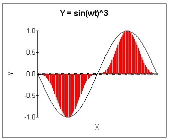
Waveshaping is a popular synthesis-and-transformation technique that turns simple sounds into complex sounds. You can take a pure tone, like a sine wave, and transform it into a harmonically rich sound by changing its shape. A guitar fuzz box is an example of a waveshaper. The unamplified electric guitar sound is fairly close to a sine wave. But the fuzz box amplifies it and gives it sharp corners. We have seen in earlier chapters that a signal with sharp corners has lots of high harmonics. Sounds that have passed through a waveshaper generally have a lot more energy in their higher-frequency harmonics, which gives them a "richer" sound. Simple Waveshaping FormulaeA waveshaper can be described as a function that takes the original signal x as input and produces a new output signal y. This function is called the transfer function. y = f(x) This is simple, right? In fact, it’s much simpler than any other function we’ve seen so far. That’s because waveshaping, in its most general form, is just any old function. But there’s a lot more to it than that. In order to change the shape of the function (and not just make it bigger or smaller), the function must be nonlinear, which means it has exponents greater than 1, or transcendental (like sines, cosines, exponentials, logarithms, etc.). You can use almost any function you want as a waveshaper. But the most useful ones output zero when the input is zero (that’s because you usually don’t want any output when there is no input). 0 = f(0) Let’s look at a very simple waveshaping function: y = f(x) = x * x * x = x3 What would it look like to pass a simple sine wave that varied from y = x3 = sin3(wt) If we plot both functions (sin(x) and the output signal), we can see that the original input signal is very round, but the output signal has a narrower peak. This will give the output a richer sound.
Figure 4.15 Waveshaping by x3. This example gives some idea of the power of this technique. A simple function (sine wave) gets immediately transformed, using simple math and even simpler computation, into something new. One problem with the y = x3 waveshaper is that for x-values outside the range –1.0 to +1.0, y can get very large. Because computer music systems (especially sound cards) generally only output sounds between –1.0 and +1.0, it is handy to have a waveshaper that takes any input signal and outputs a signal in the range –1.0 to +1.0. Consider this function: y = x / (1 + |x|) When x is zero, y is zero. Plug in a few numbers for x, like 0.5, 7.0, 1,000.0, –7.0, and see what you get. As x gets larger (approaches positive infinity), y approaches +1.0 but never reaches it. As x approaches negative infinity, y approaches –1.0 but never reaches it. This kind of curve is sometimes called soft clipping because it does not have any hard edges. It can give a nice "tubelike" distortion sound to a guitar. So this function has some nice properties, but unfortunately it requires a divide, which takes a lot more CPU power than a multiply. On older or smaller computers, this can eat up a lot of CPU time (though it’s not much of a problem nowadays). Here is another function that is a little easier to calculate. It is designed for input signals between –1.0 and +1.0. y = 1.5x - 0.5x3 |
||
| |
||
|
|
This applet plays a sine wave through various waveshaping formulae. |
|
| |
||
Chebyshev PolynomialsA transfer function is often expressed as a polynomial, which looks like: y = f(x) = d0 + d1x + d2x2 + d3x3 + ... + dNxN The highest exponent N of this polynomial is called the "order" of the polynomial. In Applet 4.9, we saw that the x2 formula resulted in a doubling of the pitch. So a polynomial of order 2 produced strong second harmonics in the output. It turns out that a polynomial of order N will only generate frequencies up to the Nth harmonic of the input sine wave. This is a useful property when we want to limit the high harmonics to a value below the Nyquist rate to avoid aliasing. Back in the 19th century, Pafnuty Chebyshev discovered a set of polynomials known as the Chebyshev polynomials. Mathematicians like them for lots of different reasons, but computer musicians like them because they can be used to make weird noises, er, we mean music. These Chebyshev polynomials have the property that if you input a sine wave of amplitude 1.0, you get out a sine wave whose frequency is N times the frequency of the input wave. So, they are like frequency multipliers. If the amplitude of the input sine wave is less than 1.0, then you get a complex mix of harmonics. Generally, the lower the amplitude of the input, the lower the harmonic content. This gives musicians a single number, sometimes called the distortion index, that they can tweak to change the harmonic content of a sound. If you want a sound with a particular mixture of harmonics, then you can add together several Chebyshev polynomials multiplied by the amount of the harmonic that you desire. Is this cool, or what? Here are the first few Chebyshev polynomials: T0(x) = 1 You can generate more Chebyshev polynomials using this recursive formula (a recursive formula is one that takes in its own output as the next input): Tk+1(x) = 2xTk(x) – Tk–1(x) Table-Based WaveshapersDoing all these calculations in realtime at audio rates can be a lot of work, even for a computer. So we generally precalculate these polynomials and put the results in a table. Then when we are synthesizing sound, we just take the value of the input sine wave and use it to look up the answer in the table. If you did this during an exam it would be called cheating, but in the world of computer programming it is called optimization. One big advantage of using a table is that regardless of how complex
the original equations were, it always takes the same amount of time to
look up the answer. You can even draw a function by hand without using
an equation and use that hand-drawn function as your transfer function. |
||
| |
||
|
|
This applet plays sine waves through polynomials and hand-drawn waves. |
|
| |
||
Don Buchla’s SynthesizersDon Buchla, a pioneering designer of synthesizers, created a series of
instruments based on digital waveshaping. One such instrument, known as
the Touche, was released in 1978. It had 16 digital oscillators
that could be combined into eight voices. The Touche had extensive programming
capabilities and had the ability to morph one sound into another. Composer
David Rosenboom worked with Buchla and developed much of the software
for the Touche. Rosenboom produced an album in 1981 called Future Travel
using primarily the Touche and the Buchla 300 Series Music System. |
||
| |
||
|
|
Now that you know a lot about waveshaping, Chebyshev polynomials, and transfer functions, we’ll show you what happens when the information gets into the wrong hands! These soundfiles are two recordings done in the mid-1980s, at the Mills College Center for Contemporary Music, by one of our authors (Larry Polansky). They use an highly unusual live, interactive computer music waveshaping system. "Toyoji Patch" was a piece/software/installation written originally for trombonist and composer Toyoji Tomita to play with. It was a real-time feedback system, which fed live audio into the transfer function of a set of six digital waveshaping oscillators. The hardware was an old S-100 68000-based computer system running the original prototype of a computer music language called HMSL, including a GUI and set of instrument drivers and utilities for controlling synthesizer designer Don Buchla’s 400 series digital waveshaping oscillators. The system could be used with or without a live input, since it made use of an external microphone to feed back its output to itself. The audio time domain signal used a transfer function to modify itself, but you could also alter Chebyshev coefficients in realtime, redraw the waveform, and control a number of other parameters. Both of these sound excerpts feature the amazing contemporary flutist Anne LaBerge. In the first version, LaBerge is playing but is not recorded. She is in another room, and the output of the system is fed back into itself through a microphone. By playing, she could drastically affect the sound (since her flute went immediately into the transfer function). However, although she’s causing the changes to occur, we don’t actually hear her flute. In the second version, LaBerge is in front of the same microphone that’s used for feedback and recording. In both versions, Polansky was controlling the mix and the feedback gain as well as playing with the computer. |
|
| <-- Back to Previous Page | Next Section --> |
©Burk/Polansky/Repetto/Roberts/Rockmore. All rights reserved.