|
| <-- Back to Previous Page | TOC | Next Section --> |
Chapter 1: The Digital Representation of Sound,
|
||
|
|
Sound is a complex phenomenon involving physics and perception. Perhaps the simplest way to explain it is to say that sound involves at least three things:
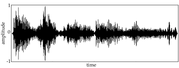
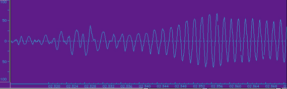
All things that make sound move, and in some very metaphysical sense, all things that move (if they don’t move too slowly or too quickly) make sound. As things move, they "push" and "pull" at the surrounding air (or water or whatever medium they occupy), causing pressure variations (compressions and rarefactions). Those pressure variations, or sound waves, are what we hear as sound. Sound is often represented visually by figures, as in Figures 1.1 and 1.2.
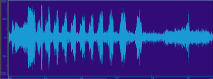
Figure 1.1 Most sound waveforms end up looking pretty much alike. It’s hard to tell much about the nature of this sound from this sort of time-domain plot of a sound wave.
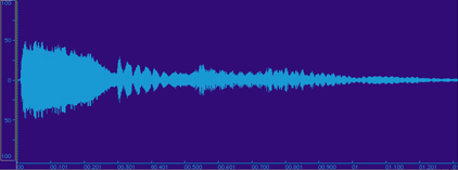
Figure 1.2 Minute portion of the sound wave file from Figure 1.1, zoomed in many times. Figures 1.1 and 1.2 are often called functions. The concept of function is the simplest glue between mathematical and musical ideas. Sound as a FunctionMost of you probably have a favorite song, something that reminds you of a favorite place or person. But how about a favorite function? No, not something like a black-tie affair or a tailgate party; we mean a favorite mathematical function. In fact, songs and functions aren’t so different. Music, or more generally sound, can be described as a function. Mathematical functions are like machines that take in numbers as raw material and, from this input, produce another number, which is the output. |
|
|
|
There are lots of different kinds of functions. Sometimes functions operate by some easily specified rule, like squaring. When a number is input into a squaring function, the output is that number squared, so the input 2 produces an output of 4, the input 3 produces an output of 9, and so on. For shorthand, we’ll call this function s. s(2) = 22 = 4 The last expression is really just an abbreviation that says for any number given as input to s, the number squared is the output. If the input is x, then the output is x2. Sometimes the input/output relation may be easy to describe, but often the actual cause and effect may be more complicated. For example, review the following function.
Once again, for shorthand we can abbreviate this and call the function f. f(5) = room temperature at 5 minutes after 8 A.M.
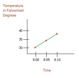
You can see how this temperature function is a little like our previous sound amplitude graphs. The easiest way to understand the temperature function is according to its graph, the picture that helps us visualize the function. The two axes are the input and output. If an input is some number x units from 0 and the output is f(x) units (which could be a positive or negative number), then we place a mark at f(x) units above x. Assume the following:
f(0) = 30
Figure 1.3 shows what happens when we graph these three temperatures. (Note that we’ll leave the x-axis in real time, but to be more precise we probably should have written 0, 5, and 10 there!) We’ll join these marks by a straight line.
Figure 1.3 So how do we get a function out of sound or music? A Kindergarten ExampleImagine an entire kindergarten class piled on top of a trampoline in your neighbor’s backyard (yes, we know this would be dangerous!). The kids are jumping up and down like maniacs, and the surface of the trampoline is moving up and down in a way that is seemingly impossible to analyze. Suppose that before the kids jump on the trampoline, we paint a fluorescent yellow dot on the trampoline and then ask the kids not to jump on that dot so that we can watch how it moves up and down. The surface of the trampoline is initially at rest. The class climbs on. We take a stopwatch out of our pocket and yell "Go!" while simultaneously pressing the start button. As the kids go crazy, our job is to measure at each possible instant how far the yellow dot has moved from its rest position. If the dot is above the initial position, we measure it as positive (so a displacement of 3 cm up is recorded as +3). If the displacement is below the rest position, we measure it as negative (so a displacement of 3 cm down is recorded as -3). So follow the bouncing dot! It rises, then falls, sometimes a lot, sometimes a little, again and again. If we chart this bouncing dot on a moving piece of paper, we get the kind of function (of pressure, or deformation or perturbation) that we’ve been talking about. Let’s return to the idea of writing down a list of numbers corresponding to a set of times. Now we’re going to turn that list into the graph of a mathematical function! We’ll call that function F. On the horizontal line (the x-axis), we mark off the equally spaced numbers 1, 2, 3, and so on. Then we mark off on the vertical axis (the y-axis) the numbers 1, 2, 3, and so on, going up, and -1, -2, -3, and so on, going down. The numbers on the x-axis stand for time, and on the y-axis the numbers represent displacement. If at time N we recorded a displacement of 4, we put a dot at 4 units above N and we say that F(N) = 4. If we recorded a displacement of -2, we put a dot at the position 2 units below N and we say F(N) = -2. Each of the values F(N) is called a sample of the function F. We’ll learn later (in Section 2.1, when we talk about sampling a waveform) that this process of "every now and then" recording the value of a displacement in time is referred to as sampling, and it’s fundamental to computer music and the storage of digital data. Sampling is actually pretty simple. We regularly inspect some continuous movement and record its position. It’s like watching a marathon on television: you don’t really need to see the whole thing from start to finish—checking in every minute or so gives you a good sense of how the race was run. But suppose you could take a measurement at absolutely every instant in time—that is, take these measurements continuously. That would give you a lot of numbers (infinitely many, in fact, because who’s to say how small a moment in time can be?). Then you would have numbers above and below every point and get a picture something like Figures 1.1 and 1.2, which appear to be continuous. Actually, calling these axes x and y is not so instructive. It is better to call the y-axis "amplitude" and the x-axis "time." The following examples let you play with the notion of pressures in time. |
|
|
|
Figure 1.4 |
|
|
|
Figure 1.5 |
|
|
|
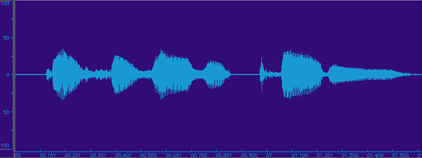
Figure 1.6 When you hear something, this is in fact the end result of a very complicated sequence of events in your brain that was initiated by vibrations of your eardrum. The vibrations are caused by air molecules hitting the eardrum. Together they act a bit like waves crashing against a big rubber seawall (or those kids on the trampoline). These waves are the result of things like speaking, plucking a guitar string, hitting a key of the piano, the wind rustling leaves, or blowing into a saxophone. Each of these actions causes the air molecules near the sound source to be disturbed, like dropping many pebbles into a pond all at once. The resulting waves are sent merrily on their way toward you, the listener, and your eagerly awaiting eardrum. The corresponding function takes as input the number representing the time elapsed since the sound was initiated and returns a number that measures how far and in what direction your eardrum has moved at that instant. But what is your eardrum actually measuring? That’s what we’ll talk about next. Amplitude and PressureIn the graphs of sound waves shown in Figures 1.1 and 1.2, time was represented on the x-axis and amplitude on the y-axis. So as a function, time is the input and amplitude (or pressure) is the output, just like in the temperature example. As we’ll point out again and again in this chapter, one way to think about sound is as a sequence of time-varying amplitudes or pressures, or, more succintly, as a function of time. The amplitude (y-)axis of the graphs of sound represents the amount of air compression (above zero) or rarefaction (below zero) caused by a moving object, like vocal chords. Note that zero is the "rest" position, or pressure equilibrium (silence). Looking at the changes in amplitude over time gives a good idea of the amplitude shape or envelope of the sound wave. Actually, this amplitude shape might correspond closely to a number of things, including:
This picture of a sound wave, as with amplitudes in time, provides a nice visual metaphor for the idea of sound as a continuous sequence of pressure variations. When we talk about computers, this graph of pressure versus time becomes a picture of a list of numbers plotted against some variable (again, time). We’ll see in Chapter 2 how these numbers are stored and manipulated. Frequency: A PreviewAmplitude is just one mathematical, or acoustical, characteristic of sound, just as loudness is only one of the perceptual characteristics of sounds. But, as we know, sounds aren’t only loud and soft. People often describe musical sounds as being "high" or "low." A bird tweeting may sound "high" to us, or a tuba may sound "low." But what are we really saying when we classify a sound as "high" or "low"? There’s a fundamental characteristic of these graphs of pressure in time that is less obvious to the eye but very obvious to the ear: namely, whether there is (or is not) a repeating pattern, and if so how quickly it repeats. That’s frequency! |
|
|
|
When we say that the tuba sounds are low and the bird sounds are high, what we are really talking about is the result of the frequency of these particular sounds—how fast a pattern in the sound’s graph repeats. In terms of waveforms, like what you saw and heard in the previous sound files, we can, for the moment, somewhat concisely state that the rate at which the air pressure fluctuates (moves in and out) is the frequency of the sound wave. We’ll learn a lot more about frequency and its related cognitive phenomenon, pitch, in Section 1.3. How Our Ears WorkMathematical functions and kids jumping on a trampoline are one thing, but what’s the connection to sound and music? Just moving an eardrum in and out can’t be the whole story! Well, it isn't. The ear is a complex mechanism that tries to make sense out of these arbitrary functions of pressure in time and sends the information to the brain. We’ve already used the physical analogy of the trampoline as our eardrum and the kids as the air molecules set in motion by a sound source. But to cover the topic more completely, we need to discuss how sounds interact, via the eardrum, with the rest of our auditory system (including the brain). Our eardrums, like microphones and speakers, are in a sense transducers—they turn one form of information or energy into another. When sound waves reach our ears, they vibrate our eardrums, transferring the sound energy through the middle ear to the inner ear, where the real magic of human hearing takes place in a snail-shaped organ called the cochlea. The cochlea is filled with fluid and is bisected by an elastic partition called the basilar membrane, which is covered with hair cells. When sound energy reaches the cochlea, it produces fluid waves that form a series of peaks in the basilar membrane, the position and size of which depend on the frequency content of the sound. Different sections of the basilar membrane resonate (form peaks) at different frequencies: high frequencies cause peaks toward the front of the cochlea, while low frequencies cause peaks toward the back. These peaks match up with and excite certain hair cells, which send nerve impulses to the brain via the auditory nerve. The brain interprets these signals as sound, but as an interesting thought experiment, imagine extraterrestrials who might "see" sound waves (and maybe "hear" light). In short, the cochlea transforms sounds from their physical, time domain (amplitude versus time) form to the frequency domain (amplitude versus frequency) form that our brains understand. Pretty impressive stuff for a bunch of goo and some hairs!
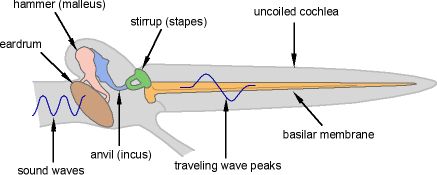
Figure 1.7 Diagram of the inner ear showing how sound waves that enter through the auditory canal are transformed into peaks, according to their frequencies, on the basilar membrane. In other words, the basilar membrane serves as a time-to-frequency converter, in order to prepare sonic information for its eventual cognition by the higher functions of the brain. Who’d have thought sound was this complicated! But keep in mind that the sound wave pressure picture is just raw data; it contains no frequency, timbral, or any other kind of information. It needs a lot of processing, organization, and consideration to provide any sort of meaning to us higher species. We’ve made the hearing process seem pretty simple, but actually there’s a lot of controversy in current auditory cognition research about the specifics of this remarkable organ and how it works. As we understand more and more about the ear, musicians and scientists gain an increasing sense of understanding how we perceive sound, and even, some believe, how we perceive music. It’s an exciting field of research, and an active one! |
|
|
|
How Do We Describe Sound?Sound can be described in many ways. We have a lot of different words for sounds, and different ways of speaking about them. For example, we can call a sound "groovy," "dark," "bright," "intense," "low and rumbly," and so on. In fact, our colloquial language for talking about sound, from a scientific viewpoint, is pretty imprecise. Part of what we’re trying to do in computer music is to try to formulate more formal ways of describing sonic phenomena. That doesn’t mean that there’s anything wrong with our usual ways of talking about sounds: our current vocabulary actually works pretty well. But to manipulate digital signals with a computer, it is useful to have access to a different sort of description. We need to ask (and answer!) the following kinds of questions about the sound in question:
Even some of these questions can be broken down into lots of smaller questions. For example, what specifically is meant by "pitch"? Taken together, the answers to these questions and others help describe the various characteristics and features that for many years have been referred to collectively as the timbre (or "color") of a sound. But before we talk about timbre, let’s start with more basic concepts: amplitude and loudness (Section 1.2). |
| <-- Back to Previous Page | Next Section --> |
©Burk/Polansky/Repetto/Roberts/Rockmore. All rights reserved.